Will Colgate Exam 3 Answers Notebook

1. What are voting classifiers in ensemble learning?

Ensemble learning combines the predictions of a number of different models in order to improve robustness of a prediction.

A well known example of an ensemble method in respect to decision trees is a random forest, where each tree in the forest is built using a random subsample (a bootstrap sample) of the training data. Features can also be randomised and chosen this way. The prediction of the random forest would then be the average of the predictions of the underlying trees.

When using a number of conceptually different machine learning models to make predictions, a voting classifier is a way to combine these different predictions in order to give an overall ensemble model prediction.

Simple majority voting is one way to make a prediction and this is known as a hard voting classifier. The algorithm simply counts the numbers of each class and the class with the highest count is the overall prediction. When there is an equal number of votes for 2 classes, you are effectively down to flipping a coin (Scikit Learn simply takes the first class in ascending order).

Alternatively, a weighted average probability can be used to determine which class should be chosen. Each model is assigned a weight. The probability of a class being chosen is calculated for each model. Weights are applied and the highest weighted average probability is then chosen. This is also known as a soft voting classifier.

2. Explain the role of the regularization parameter C in a Support Vector Machine (SVM) model. How does varying C affect the model’s bias and variance trade-off?

In the context of SVM, the parameter C is used to punish the model for misclassifying data. It would generally been seen in datasets with soft margins but a very low (or 0) value of C could even impact the accuracy of models with hard margins.

Generally speaking, a lower value for C means less importance is placed on classification error and so the margin is allowed to grow. This in turn increases the prediction error (both for training and testing data). The model would exhibit higher bias and would generally be under fitted to the data.

Contrary to this, higher values of C lead to a shrinking margin as the algorithm is punished for misclassifying points within the training data. This would result in higher variance and overfitting for very high values of C, as the model essentially would fit the training data perfectly.

3. Follow the 7-steps to model building for your selected ticker,

(a) produce a model to predict positive moves (up trend) using Random Forest Classifier.

(b) tune hyperparameters for the estimator and present the best model.

(c) investigate the prediction quality using area under ROC curve, confusion matrix and classification report.

Note: Choice and number of hyperparameters to be optimized for the best model are design choices. Use of experiment tracking tools like MLFlow is allowed [refer to Advanced Machine Learning Work- shop - II for sample implementation].

1. Ideation

The objective of the model is to successfully predict upwards trend in the movement of Schroders Plc shares. Daily data has been chosen so we are effectively trying to predict if the closing price tomorrow will be higher than today (and so, would be a signal to buy). A 1 would indicate a signal to buy (i.e. upward trend) whereas 0 would be a signal to sell (i.e. downward trend).

Small changes in price will be considered later in further detail when the relative size of the returns of the ticker I have chosen have been examined in further detail.

I chose the Schroders Plc (SDR.L) stock ticker for this analysis. As a traditional asset manager, the company is especially vulnerable to movements in wider global markets due to its fee earning model. It will be interesting to see if any discernable patterns emerge from analysing returns over the period.

Data Collection

Data has been collected using yfinance. This has been incorporated into a class object with standard functionality that can be performed on the data.

Data returned from yfinance is in the below format:

Column	Description
Open	Opening price of the security
Close	Closing price of the security
High	Highest traded price during the period
Low	Lowest traded price during the period
Volume	Number of shares traded in the given period
Dividends	Stock dividend events
Stock Splits	Stock split events

Data index is time series data.

# Imports
# Base
import numpy as np
import pandas as pd
# Data
from utils import TimeSeriesData

# Plotting
import matplotlib.pyplot as plt

# Preprocessing
from utils import create_features, create_dependent_variable
from sklearn.feature_selection import SelectKBest

# Metrics
from sklearn.model_selection import RandomizedSearchCV, TimeSeriesSplit
from sklearn.metrics import classification_report


# Model
from sklearn.ensemble import RandomForestClassifier

# Classification
from utils import FinancialTimeSeriesClassifier

import warnings
warnings.filterwarnings('ignore')

# Create an object for time series data and examine head of table
schroders = TimeSeriesData('SDR.L', period='5y')
schroders.head()

	Open	High	Low	Close	Volume	Dividends	Stock Splits
Date
2018-10-22 00:00:00+01:00	386.750454	392.421689	382.462433	382.462433	3104976	0.0	0.0
2018-10-23 00:00:00+01:00	376.929537	379.695987	366.278687	366.278687	7284688	0.0	0.0
2018-10-24 00:00:00+01:00	364.895415	371.119934	360.745728	360.745728	4292929	0.0	0.0
2018-10-25 00:00:00+01:00	360.745729	368.906796	357.702637	368.076843	2575141	0.0	0.0
2018-10-26 00:00:00+01:00	362.682283	363.788878	356.181121	360.884094	5325470	0.0	0.0

5 years of data was chosen as it actually gave a better predictive power than 10 years. This is likely due to data further back in time having less relevance on today.

Exploratory Data Analysis (EDA)

schroders.plot()

Just eyeballing the price and volume data over the past 5 years gives us the following insights:

• There were large falls in the price in early 2020 (covid lockdown) & late 2022 (global rate rises) and strong growth from early 2020 to late 2021 (initial covid recovery). This indicates that the price of this particular stock moves in line with the market more generally which is to be expected given they are an active fund manager and earn fees based on a % of AUM they manage.
• Volumes were much lower in the 2020 crash, suggesting that people took a wait and see mentality. This is contrasted by 2022 and 2023 where rate rises saw much more volume over a protracted period, possibly due to debt securities offering a better return with less risk.

schroders.describe()

	Open	High	Low	Close	Volume	Dividends	Stock Splits
count	1262.000000	1262.000000	1262.000000	1262.000000	1.262000e+03	1262.000000	1262.000000
mean	455.925056	461.279874	450.760267	456.121106	2.374145e+06	0.079810	0.001864
std	63.027873	62.377632	63.082345	62.649890	2.038807e+06	0.958721	0.046816
min	251.844900	308.997103	246.937895	302.791199	1.318820e+05	0.000000	0.000000
25%	415.589918	422.027350	411.341995	416.405441	1.270400e+06	0.000000	0.000000
50%	447.678484	451.860430	441.964362	447.684662	1.878035e+06	0.000000	0.000000
75%	501.294655	505.882132	496.712724	501.525948	2.788922e+06	0.000000	0.000000
max	607.796920	609.510336	597.516458	602.968262	3.093360e+07	15.000000	1.176471

The data looks to be complete for the past 10 years. One issue looks to be that Volume has a minimum of nil. This is unlikely in practice so suggests an error in the data.

# Check how many entries have nil volume
schroders.df[schroders.df['Volume']==0]

	Open	High	Low	Close	Volume	Dividends	Stock Splits
Date

Cleaning Data

The data received from yfinance is generally already cleaned but I have checked for missing values below to make sure.

schroders.df.isnull().sum()

Open            0
High            0
Low             0
Close           0
Volume          0
Dividends       0
Stock Splits    0
dtype: int64

As expected, there are no null values in the data. The last piece of cleaning is to replace the nil volume data. This will be done by simple backfill from the day before.

schroders.df['Volume'].replace(0, method='ffill', inplace=True)

# Check how many entries have nil volume
schroders.df[schroders.df['Volume']==0]

	Open	High	Low	Close	Volume	Dividends	Stock Splits
Date

Transform Data

At this step, features will be created, scaled (if required) and selected through experimentation and finance domain knowledge to give a final set of features to use in our model. I have focused on coding up a variety of technical indicators that a day trader might use to predict momentum. After we have created these and our variable to be predicted, we will spend some time choosing which features should be retained in the model.

Feature Creation

A variety of features were created in that represent standard trading metrics. The code in utils.py clearly demonstrates how each of these features are calculated.

# Create thr features
X = create_features(schroders)
X.head()

	Close	Dividends	EMA14	EMA28	EMA7	GAP	GAP14	GAP28	GAP7	HL	...	UB14	UB28	UB7	VCHG14	VCHG28	VCHG7	VMA14	VMA28	VMA7	Volume
Date
2018-11-29 00:00:00+00:00	358.255951	0.0	354.607597	358.950704	354.640855	0.003881	0.001873	0.000093	0.001614	0.023763	...	365.452703	374.698429	366.070155	0.371611	-0.010276	-0.189630	1.090516	0.924380	0.998169	3073070
2018-11-30 00:00:00+00:00	349.541565	0.0	353.932126	358.301798	353.366032	0.001930	0.000943	0.000679	0.001248	0.027723	...	365.180057	374.061515	365.347688	0.901636	-0.488976	0.287879	1.264457	1.164329	1.164208	3722652
2018-12-03 00:00:00+00:00	358.255951	0.0	354.508636	358.298636	354.588512	0.012663	0.001987	0.001266	0.002485	0.019585	...	364.736784	373.924011	363.643381	-0.297851	-0.571113	0.476936	0.637466	0.592079	0.560905	1841182
2018-12-04 00:00:00+00:00	352.031464	0.0	354.178347	357.866417	353.949250	-0.003089	0.002068	0.001156	0.002331	0.022030	...	363.877200	372.905322	363.216857	-0.347485	-0.426590	-0.433873	0.521381	0.480909	0.473143	1476611
2018-12-05 00:00:00+00:00	347.051819	0.0	353.228143	357.120583	352.224892	-0.013752	0.000892	0.001188	-0.000592	0.032494	...	363.844208	372.720424	363.414475	-0.268894	-0.675285	-0.613061	0.620542	0.587779	0.633555	1729258

5 rows × 51 columns

Feature EDA

In order to determine a good indicator for momentum of this stock, some further analysis of the return is required. It would not be a good indicator of upward momentum if $r_{t+1}$ is very small.

display(X['RET'].describe(percentiles=[0.05, 0.25, 0.45, 0.5, 0.55, 0.75, 0.95]))
X['RET'].plot(colormap='Dark2', title='SDR.L 10 year log return')
plt.show()

count    1234.000000
mean        0.000022
std         0.019089
min        -0.142370
5%         -0.027620
25%        -0.009038
45%        -0.001403
50%         0.000000
55%         0.001737
75%         0.009888
95%         0.028308
max         0.094883
Name: RET, dtype: float64

The plot indicates that the stock prices are essentially random with a mean return of close to zero. A good indicator of moderate to strong upward trend might be where the return breaks out of the 55th percentile. We will use this metric for calculating the dependent variable for this analysis.

y = create_dependent_variable(X, threshold=0.002)

As we are using a tree based ensemble model classifier, it would be prudent to perform feature importance analysis based on a decrease in impurity or entropy.

forest_gini = RandomForestClassifier(random_state=0)
forest_entropy = RandomForestClassifier(random_state=0, criterion='entropy')
display(forest_gini.fit(X, y))
forest_entropy.fit(X, y)

RandomForestClassifier(random_state=0)

In a Jupyter environment, please rerun this cell to show the HTML representation or trust the notebook.
On GitHub, the HTML representation is unable to render, please try loading this page with nbviewer.org.

RandomForestClassifier(criterion='entropy', random_state=0)

In a Jupyter environment, please rerun this cell to show the HTML representation or trust the notebook.
On GitHub, the HTML representation is unable to render, please try loading this page with nbviewer.org.

# Calculate the importances and sort them high to low for display
gini_importances = forest_gini.feature_importances_
entropy_importances = forest_entropy.feature_importances_
gini_importances = pd.Series(gini_importances, index=X.columns)
gini_importances.sort_values(inplace=True, ascending=False)
entropy_importances = pd.Series(entropy_importances, index=X.columns)
entropy_importances.sort_values(inplace=True, ascending=False)

fig, ax = plt.subplots(2, 1)
gini_importances.plot.bar(ax=ax[0], color='green')
entropy_importances.plot.bar(ax=ax[1], color='green')
ax[0].set_title("Decrease in impurity")
ax[1].set_title("Decrease in entropy")
ax[0].set_ylabel("Mean decrease", y=-0.5)
fig.tight_layout()

It is clear from the above that Sign, Dividends and Stock Splits add very little to the reduction in impurity/entropy as the trees are built and can safely be removed.

The remainder all contribute a material amount to building the tree and will be left in for now. When we tune the hyperparameters, we will experiment with different random subsets of features using the max_features hyperparameter.

X.drop(['Dividends', 'Stock Splits', 'SIGN'], axis=1, inplace=True)
X.shape

(1234, 48)

The data still has 48 features and some features look very similar in their reduction in impurity. This could mean that certain features are correlated. To explore reducing the number od features/dimensions further, I will use one more filter method, K-best.

Using Scikit Learn's SelectKBest to choose the the k best features to use.

kbest = SelectKBest(k='all')
kbest.fit(X, y)
# Print the scores in descending order
scores_df = pd.DataFrame(kbest.scores_, index=X.columns, columns=['F Score']).sort_values('F Score',ascending=False)
scores_df.plot(kind='bar', fontsize=8, colormap='Dark2', title='F Statistic Score')

<Axes: title={'center': 'F Statistic Score'}>

There is a sharp drop off contribution to the after UB28 so we will use this subset of features only.

# Find score of UB28
lower_limit = scores_df.loc['UB28'].values[0]
# Filter the dataframe and take teh index labels
scores_df = scores_df[scores_df['F Score'] >= lower_limit]
labels = list(scores_df.index)
X = X[labels]
X.shape

(1234, 30)

Model

The model stipulated in the question is the Random Forest Classifier. However, I have coded a classifier class that is flexible enough to accommodate a number of different models to better facilitate experimentation with different models at a later date.

Hyperparameter tuning will be accomplished using Grid Search with cross validation using forward chaining to keep the time series structure of the data in tact.

Note that as the Random Forest is essentially a grouping of Decision Trees, there is no need to scale the data (although the option has been included so the classifier can be used on other models).

Firstly, we will make a prediction on "out of the box" settings to see what we are dealing with.

clf = FinancialTimeSeriesClassifier(X, y)
clf.fit_predict(RandomForestClassifier(random_state=45))
clf.model.get_params()

{'memory': None,
 'steps': [('classifier', RandomForestClassifier(random_state=45))],
 'verbose': False,
 'classifier': RandomForestClassifier(random_state=45),
 'classifier__bootstrap': True,
 'classifier__ccp_alpha': 0.0,
 'classifier__class_weight': None,
 'classifier__criterion': 'gini',
 'classifier__max_depth': None,
 'classifier__max_features': 'sqrt',
 'classifier__max_leaf_nodes': None,
 'classifier__max_samples': None,
 'classifier__min_impurity_decrease': 0.0,
 'classifier__min_samples_leaf': 1,
 'classifier__min_samples_split': 2,
 'classifier__min_weight_fraction_leaf': 0.0,
 'classifier__n_estimators': 100,
 'classifier__n_jobs': None,
 'classifier__oob_score': False,
 'classifier__random_state': 45,
 'classifier__verbose': 0,
 'classifier__warm_start': False}

out_of_box = classification_report(clf.y_test, clf.y_pred_test)
print(out_of_box)

              precision    recall  f1-score   support

           0       0.58      0.69      0.63       144
           1       0.42      0.31      0.36       103

    accuracy                           0.53       247
   macro avg       0.50      0.50      0.49       247
weighted avg       0.51      0.53      0.52       247

clf.plot_confusion_matrix()

clf.plot_roc_curve()

It is clear that with the initial parameters set, our model predicts no better than random. Now we will move onto hyperparameter tuning and cross validation to attempt to increase the predictive power of the model.

Cross validation is where the training data is split into small sets and part of the data is held out for validation. Classical cross validation assumes data samples are independent and identically distributed. This isn't the case with a time series, where the data exhibits autocorrelation. To preserve this order, splitting the data using forward chaining will be used. Each successive training set will be a superset of those that came before it as demonstrated in the picture below.

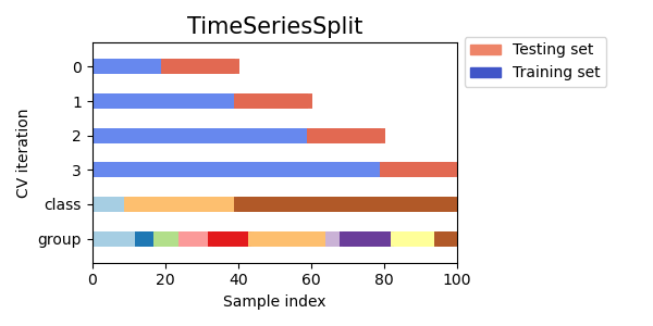
Source: Scikit Learn

The example picture above uses 4 splits the default of 5 have been used below.

# Create a time series cross validation split.
time_series_cv = TimeSeriesSplit(gap=1)

For parameters, we will focus on the below and implement a parameter grid with sensible values.

Hyperparameter	Description
max_depth	This defines how deep each tree can go. In theory, random forest should grow until all nodes are pure but we will experiment with this to see.
min_sample_split	This defines how many samples at node are allowed to be considered pure by the algorithm.
max_leaf_nodes	Only grow trees to a maximum of these leaf nodes.
min_samples_leaf	The minimum number of samples required to be at a leaf node.
n_estimators	Number of trees in the forest.
max_features	Number of features to consider when looking at the best split.
criterion	The criteria for splitting a tree (either gini, entropy or log_loss)
max_samples	the number of samples to draw from X to train each base estimator.

Due to memory concerns, a randomized search will be used.

param_grid = {
    'classifier__criterion': ['gini', 'entropy', 'log_loss'],
    'classifier__max_features': ['sqrt', 'log2', None] + list(np.arange(1, X.shape[1], 1)),
    'classifier__max_depth': [None] + list(np.arange(2, 25, 1)),
    'classifier__max_leaf_nodes': [None] + list(np.arange(10, 501, 50)),
    'classifier__min_samples_leaf': np.arange(1, 11, 1),
    'classifier__n_estimators': np.arange(50, 1001, 50),
    'classifier__min_samples_split': np.arange(2, 11, 1)
}
gs = RandomizedSearchCV(clf.model, param_grid, n_iter=500, scoring='roc_auc', n_jobs=-1, cv=time_series_cv, verbose=1, random_state=45)
gs.fit(clf.X_train, clf.y_train)

Fitting 5 folds for each of 500 candidates, totalling 2500 fits

RandomizedSearchCV(cv=TimeSeriesSplit(gap=1, max_train_size=None, n_splits=5, test_size=None),
                   estimator=Pipeline(steps=[('classifier',
                                              RandomForestClassifier(random_state=45))]),
                   n_iter=500, n_jobs=-1,
                   param_distributions={'classifier__criterion': ['gini',
                                                                  'entropy',
                                                                  'log_loss'],
                                        'classifier__max_depth': [None, 2, 3, 4,
                                                                  5, 6, 7, 8, 9,
                                                                  10, 11, 12,
                                                                  13, 14, 15,
                                                                  16, 17, 18,
                                                                  19, 20, 2...
                                        'classifier__max_leaf_nodes': [None, 10,
                                                                       60, 110,
                                                                       160, 210,
                                                                       260, 310,
                                                                       360, 410,
                                                                       460],
                                        'classifier__min_samples_leaf': array([ 1,  2,  3,  4,  5,  6,  7,  8,  9, 10]),
                                        'classifier__min_samples_split': array([ 2,  3,  4,  5,  6,  7,  8,  9, 10]),
                                        'classifier__n_estimators': array([  50,  100,  150,  200,  250,  300,  350,  400,  450,  500,  550,
        600,  650,  700,  750,  800,  850,  900,  950, 1000])},
                   random_state=45, scoring='roc_auc', verbose=1)

In a Jupyter environment, please rerun this cell to show the HTML representation or trust the notebook.
On GitHub, the HTML representation is unable to render, please try loading this page with nbviewer.org.

gs.best_params_

{'classifier__n_estimators': 250,
 'classifier__min_samples_split': 6,
 'classifier__min_samples_leaf': 7,
 'classifier__max_leaf_nodes': 110,
 'classifier__max_features': 21,
 'classifier__max_depth': 2,
 'classifier__criterion': 'entropy'}

clf.fit_predict(RandomForestClassifier(
    random_state=45, 
    criterion=gs.best_params_['classifier__criterion'], 
    max_features=gs.best_params_['classifier__max_features'],
    n_estimators=gs.best_params_['classifier__n_estimators'],
    min_samples_split=gs.best_params_['classifier__min_samples_split'],
    max_leaf_nodes=gs.best_params_['classifier__max_leaf_nodes'],
    max_depth=gs.best_params_['classifier__max_depth'],
    min_samples_leaf=gs.best_params_['classifier__min_samples_leaf']
    ))

Validation

clf.plot_confusion_matrix()

clf.plot_roc_curve()

print('Tuned model')
print(classification_report(clf.y_test, clf.y_pred_test))
print('Original model')
print(out_of_box)

Tuned model
              precision    recall  f1-score   support

           0       0.59      0.85      0.70       144
           1       0.45      0.17      0.24       103

    accuracy                           0.57       247
   macro avg       0.52      0.51      0.47       247
weighted avg       0.53      0.57      0.51       247

Original model
              precision    recall  f1-score   support

           0       0.58      0.69      0.63       144
           1       0.42      0.31      0.36       103

    accuracy                           0.53       247
   macro avg       0.50      0.50      0.49       247
weighted avg       0.51      0.53      0.52       247

Although the overall accuracy fo the model accuracy has improved by 0.04 and has correctly classified 56% of days, the models predictive power is only slightly better than random. This is further demonstrated by the confusion matrix and ROC curve.

However, the precision of "1" (i.e. predicting an upward trend) is no better than a coin flip with only 17% of positive cases being caught. All in all, I wouldn't use my own money to test this strategy....